EPOW - Ecology Picture of the Week

Give the 'Roos a Brake!

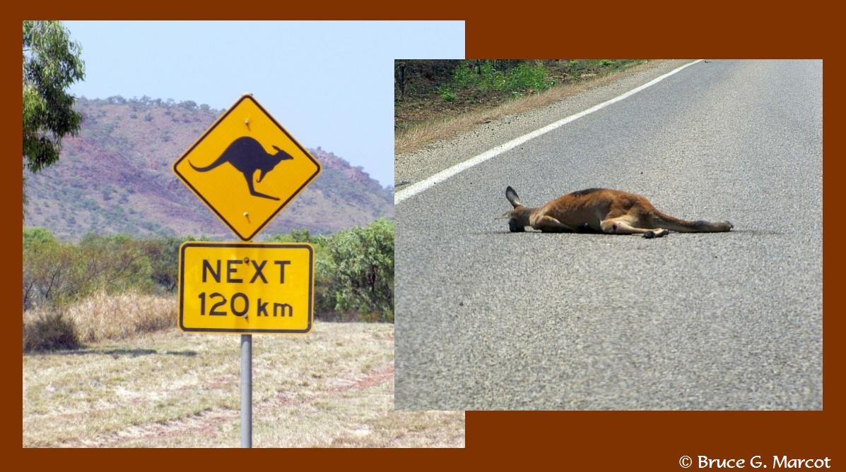
Red Kangaroo (Macropus rufus), Family Macropodidae
Queensland Outback, Australia

Explanation:  So there we were, my Australian 'mate and me, driving some 9,234 km (5,737 miles) across the Australian Outback (and back) ... doing our best to stay alert, awake, and watchful of birds and other wildlife en route ... 

... when I had the brilliant idea of counting road-kills.

So on the spot, I devised a methodology of counting all the road-kill wildlife -- kangaroos, wallabies, wallaroos, whatever fell victim to tire and grill -- on my (passenger) side of the vehicle, in five 1-km increments each interspersed with 1-km segments of not counting (to help extend each counting transect and ward off "count fatigue").  

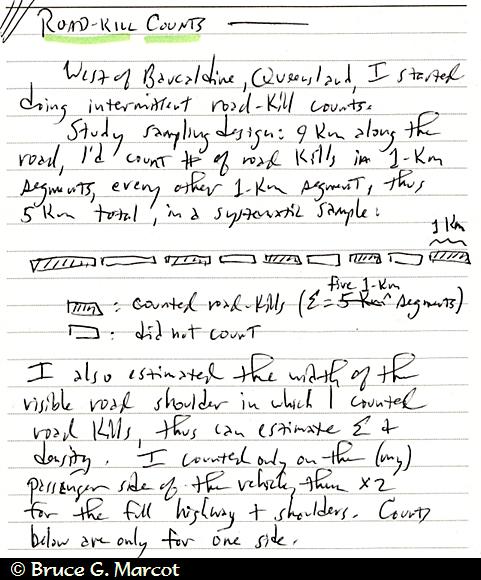
Here's an entry from my field journal describing our methods of counting road-kill animals along the endless Outback highways of central Australia.

I would record the counts in each of the 1-km "count" segments, as the driver -- the wonderful engineer and wildlife photographer Deane Lewis -- would alert me as to the start and end of each 1-km segment from his odometer.  

So each transect stretched 9 km, with 5 km having specific counts.  

Eventually, we conducted these counts along 14 such 9-km transects (thus, 126 km of count transects), totaling 70 km count-segments.  We spaced each transect more or less evenly from north of Mataranka (south of Darwin), Northern Territory, to east of Barcaldine (northwest of Brisbane), Queensland (see map below).  

We also estimated the width of the transect alongside and extending onto the road shoulder.  So knowing the width and the length of each count transect, I calculated its total area, and thus a density of numbers of road-kill animals per square kilometer of highway shoulder.  

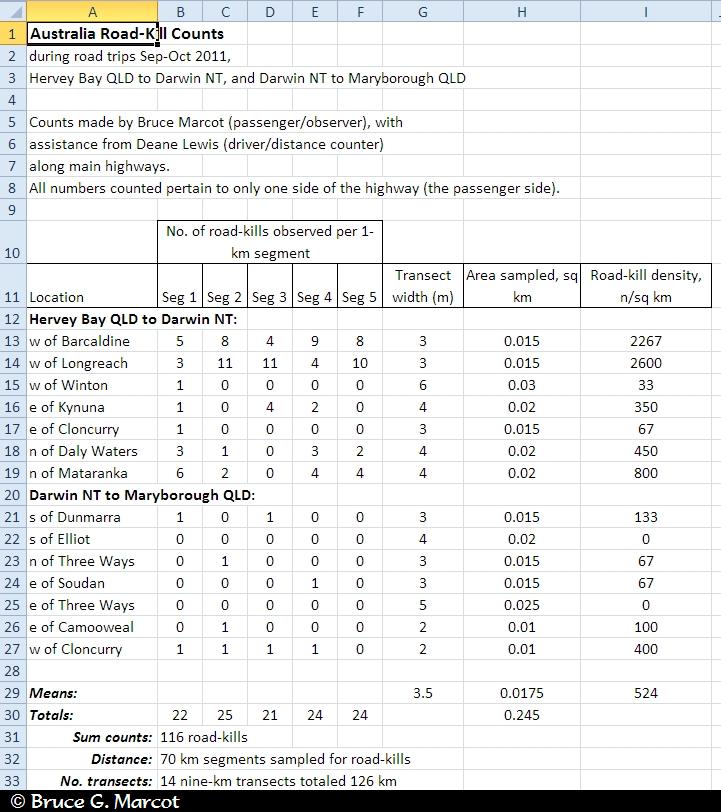
Here's the calculation sheet I developed to convert the raw counts of road-kills to density of road-kills (number of road-kills per square kilometer of highway shoulder).

The raw-count figures are only for one side of the highway.

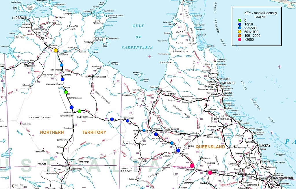
So what did we find?

I counted a total of 116 road-kills, on just my passenger side of the highway.  Doubling the counts (assuming an average of an equal number of road-kills on the other side of the highway that I did not count during our transects), there would have been a total of 232 road-kills.  

Along the 70-km of count-segments, this doubled number averages out to about 3.3 road kills per km of highway (or about 5.5 road kills per mile).  

Account for width of the transects and total area, this also averaged 1,048 road-kills per square kilometer (2,714 per square mile) of highway shoulder!

This seems like rather massive carnage to us ... 

But it wasn't evenly distributed across the landscape.  

I then plotted the location of each transect on a road map, making it clearer that the highest densities of road kills (the red and yellow dots on the map, below) occurred in northern Northwest Territory and as we approached eastern Queensland:

Click on this map for a larger version.  
Note the key to densities in the upper-right corner;
green and blue dots are the lowest densities,
and red is the highest.

So what could be affecting our counts?  We came up with a list of possibilities, including:

• highway traffic density -- especially at dusk and dawn (and perhaps at night) when many of the animals are most active, out feeding

• age class of the animals -- perhaps dispersing juveniles were more apt to wander and get hit by vehicles

• different numbers of road-kills on each side of the highway -- perhaps there had been greater traffic flowing one direction

• different numbers of animal active along roads during different seasons -- wet & dry, hot & cooler

• habitat -- particularly the presence, amount, quality, and dispersion pattern of suitable habitat along the highways, for each species (this is particularly evident in the results map, above, where lowest densities occurred in the most arid portions of the Outback route in eastern Queensland and southern Northern Territory).

Also, I counted all observable road kills.  This means:

• I may have missed some that "slipped by" (if I got out and walked a sample of each transect segment and did an absolute total count, I could have developed an "index of detectability" and corrected my counts upward for those I missed at highway speed); and

• I counted road kills of all "ages."  That is, I have no idea how long any given road kill had been lying there.  So I can't calculate a rate of vehicle collisions per unit time, only per unit length and area.  I don't know how long it took for all those road kills to "pile up," so to speak.

• I also don't know anything about differential decay rates of road-kill carcasses of different species and sizes of animals.  Do larger carcasses, such as the red kangaroo in this week's main photo decay or disintegrate slower than, say, carcasses of raptors?  

• Some animals may have been hit and not killed outright, and then jumped, crawled, or slithered off into the bush where they died undetected (thanks, John Laurence, for this idea).

• Also, disintegration rates of carcasses likely are influenced by how many times they are hit by vehicles, the speed and mass of the vehicle, the effect of scavengers, weather, and other factors.  

So what are the conclusions?

There seem to be more road kills along the parts of our Outback route that are nearer to major city centers (Darwin, Brisbane).  This may be, in turn, correlated with density of vehicle traffic and with quality of adjacent habitats.  

People may be driving too fast for conditions during the time of day or during seasons when wildlife are more active, crossing or moving along roadways.  

But we don't know if the numbers of road kills we counted (and extrapolated) are representative of other years and seasons ... nor if the numbers are having a significantly adverse effect on the populations of each of these wildlife species.

Despite all these unknowns, results of these kinds of studies can be used to build models of wildlife population distributions, dispersal, & source-sink dynamics (Kanda et al. 2009).

And as researchers always love to conclude in their publications, "more research is needed!"
  

A bumper sticker I picked up on my previous visit to Australia.
 

 
Acknowledgment:  
   My thanks to mate & colleague Deane Lewis, driver & engineer extraordinaire & creator and maintainer of OwlPages.com.

Information:
     Gunson, K. E., G. Mountrakis, and L. J. Quackenbush. 2011. Spatial wildlife-vehicle collision models: A review of current work and its application to transportation mitigation projects. Journal of Environmental Management 92(4):1074-1082.
     Jaeger, J. A. G., J. Bowman, J. Brennan, L. Fahrig, D. Bert, J. Bouchard, N. Charbonneau, K. Frank, B. Gruber, and K. T. von Toschanowitz. 2005. Predicting when animal populations are at risk from roads: an interactive model of road avoidance behavior. Ecological Modelling 185:329-348.
     Kanda, L. L., T. K. Fuller, P. R. Sievert, and R. L. Kellogg. 2009. Seasonal source–sink dynamics at the edge of a species' range. Ecology 90(6):1574-1585. 
     Roger, E., S. W. Laffan, and D. Ramp. 2011. Road impacts a tipping point for wildlife populations in threatened landscapes. Population Ecology 53(1):215-227.